From Vanilla Transformers to Modern LLMs: What Changed After the Original Transformer (Part 3)
Modern LLM Architecture (Part 3): MoE, Low-level Hardware KV Cache Optimization, and MuonClip Optimizer

This post is Part 3 of a 3-part series on modern LLM architectures. Each part can be read independently.
Part 1 talks about the techniques for improving the training stability of LLMs.
Part 2 talks about efficient architecture-level Attention Optimizations
B1) FlashAttention:
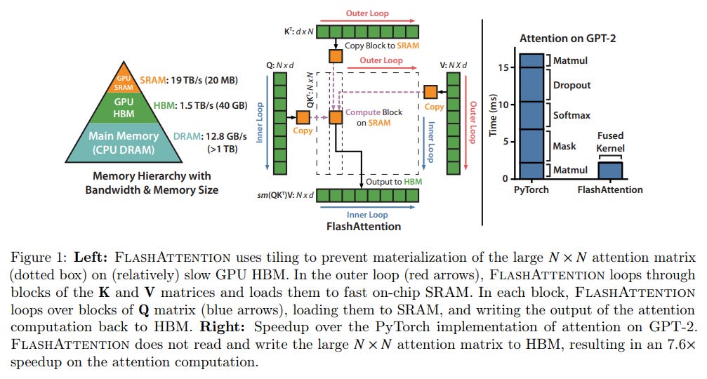
FlashAttention is a family of IO-aware exact attention algorithms that solve the “memory wall” in Transformers. Instead of storing the massive 𝑁×𝑁
attention matrix in slow GPU memory (HBM), it uses tiling to process small blocks in fast on-chip memory (SRAM).
FlashAttention-1 (2022)
The Problem: Standard attention is memory-bound; moving data between HBM and SRAM is slower than the actual math.
Key Innovation: Introduced Tiling and Recomputation. It breaks inputs into blocks to fit in SRAM and uses online softmax to compute scores incrementally. In the backward pass, it recomputes attention rather than storing it, saving massive amounts of memory.
Result: 2–4x speedup and linear (instead of quadratic) memory scaling.
FlashAttention-2 (2023)
The Problem: FlashAttention-1 had suboptimal work partitioning, leaving some GPU cores idle.
Key Innovation: Improved Parallelism. It parallelizes across the sequence length dimension (not just batch/heads) and reordered loops to reduce non-matrix-multiply overhead.
Result: Reached ~70% of A100 theoretical peak performance, nearly doubling the speed of v1.
FlashAttention-3 (2024)
The Problem: New NVIDIA Hopper (H100) hardware introduced asynchronous features that v2 couldn’t fully exploit.
Key Innovation: Asynchrony. It uses the Tensor Memory Accelerator (TMA) and WGMMA (Warpgroup Matrix Multiply-Accumulate) to overlap data movement with computation. It also introduced low-precision (FP8) support.
Result: 1.5–2x faster than v2 on H100s, reaching up to 75% of hardware utilization.
FlashAttention-4 (2025)
The Problem: Designed for the Blackwell (B200) architecture to break the “petaflop barrier”.
Key Innovation: 5-Stage Pipelining and Software Math.
Warp Specialization: It splits tasks into 5 distinct stages (Load, MMA, Softmax, Correction, Epilogue) so no part of the GPU stays idle.
Software Exponentials: It avoids bottlenecks on the GPU’s Special Function Units (SFUs) by simulating exponential math on regular CUDA cores.
Adaptive Rescaling: It only rescales values for numerical stability when “necessary,” cutting rescaling operations by 10x.
Result: The first attention kernel to achieve petaflop-scale performance; roughly 20% faster than NVIDIA’s own cuDNN on Blackwell.
FlashAttention-2 and 3 are currently the industry standards, with 3 optimized for H100s
B2) Ring Attention:
The main challenge with FlashAttention is that the memory complexity is still linear with seq_len, so scaling of sequence length is limited by the memory capacity. And also sending large matrices across devices introduces a huge communication overhead.
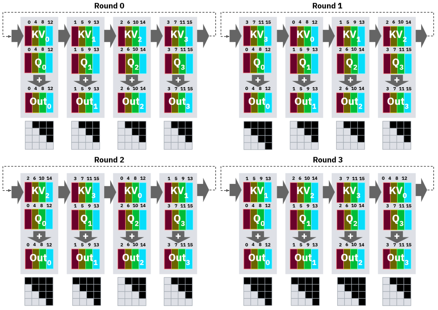
The solution is Ring Attention. Where we split Q, K, and V across the devices forming a ring structure. And key-value pairs are circulated around the ring, each device performs attention on its local queries and the received key-value blocks as shown in the below figure.
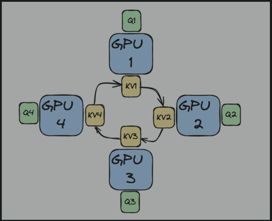
Benefit: This allows scaling memory by the number of GPUs, with communication overhead amortized for sufficiently long sequences.
B3) Stripe Attention
The issue with the Ring Attention is that, as shown in the figure below, some devices have all the tokens as masked. Hence the workload is not that distributed. So some devices stay idle during iterations, and some get fully utilized.
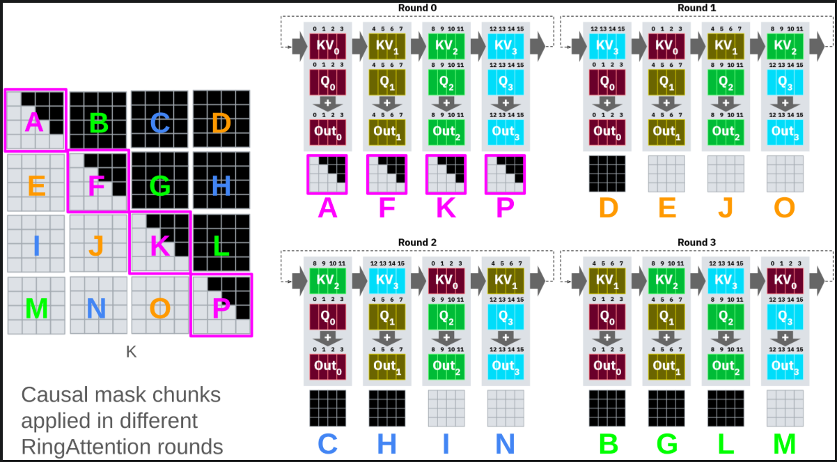
Stripe Attention solves this problem by evenly partitioning the tokens based on the residue of modulo N (number of devices) instead of just partitioning in contiguous blocks. Below is the visual representation of Stripe Attention.
B4) Paged Attention
This is an inference optimization technique. At inference, the KV cache takes a significant amount of memory to store, and in a normal manner, we store the KV cache as a contiguous memory in the storage. Due to the unpredictable output lengths from the LLM, they statically allocate a chunk of memory for a request based on the request’s maximum possible sequence length, irrespective of the actual input or eventual output length of the request. This is a pure memory waste. Although it is used later, the space used to reserve these large chunks of blocks could be used for processing other requests.
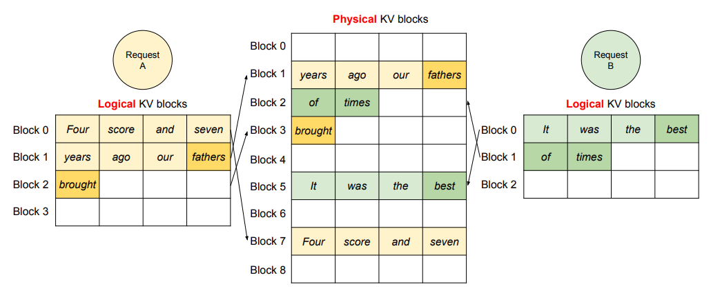
Paged Attention solves this by using Pagination, the concept that is already in use in Operating Systems. Instead, PagedAttention:
Allows storing continuous keys and values in non-contiguous memory space.
Partitions the KV cache of each sequence into KV blocks. Each block contains the key and value vectors for a fixed number of tokens, which is known as the block size, as shown in the figure.
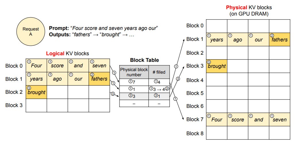
The attention computation is done block-by-block wise, and all the scores are gathered at the end.
B5) Radix Attention
In the traditional LLM serving, it computes the KV cache for each new prompt it receives, i.e., it doesn’t have any way of knowing whether a prompt sent by the user is the same as other prompt recieved before by any user. Hence, it computes the kV cache for each prompt, which is a waste of computation.
Radix Attention fixes this by storing common KV cache prefixes in a Radix Tree and sharing it with multiple calls across multiple sessions and users, hence improving the efficiency dramatically and reducing the computational cost.
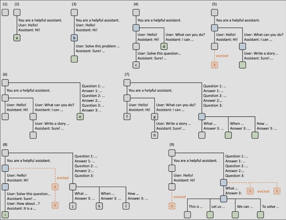
The radix Tree is as shown in the figure. At each time step the new prompt request comes in and if there is no similar prefix as the prompt, then it will be added as a new branch of the tree. As the new request comes in, if the request is same, then it will use that KV cache from the tree otherwise, a new branch is created. From time to time, the KV cache that is at a leaf node is evicted from the branch to keep a check on the total memory available.
8. MoE
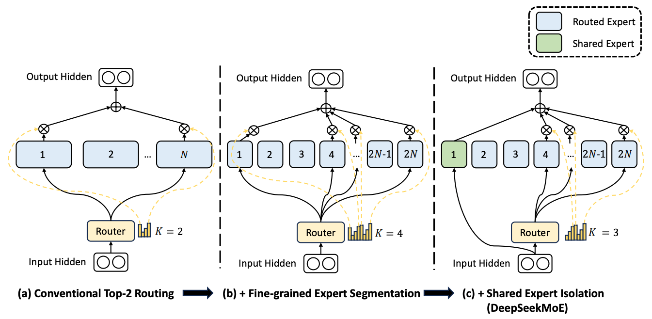
We replace FFN block in each layer with the MoE block as shown in the architecture figure at the beginning.
The MoE block consists of several smaller FFNs which are called experts. And the input is routed to the experts based on the routing function. Out af all the experts, the input is routed to onlly a few which are called the active experts. And the router determines which experts to send the input to. In some variations, there is always 1 or 2 experts that are always active, which is known as a shared expert.
Why MoE is so popular and what are its advantages?
It is faster to train MoEs: The same performance can be reached with fewer training steps
Better performance at the same amount of activated parameters as compared to non-MoEs
Parallelizable to many devices
10. MuonClip Optimizer:
Muon (MomentUm Orthogonalized by Newton-Schulz) is a specialized neural network optimizer designed to accelerate the training of large-scale models, particularly Large Language Models (LLMs). Unlike standard element-wise optimizers like AdamW, Muon leverages the matrix structure of weight layers to ensure more uniform updates across parameter space, significantly improving compute efficiency.
Orthogonalization: It transforms raw momentum into an orthogonal matrix. This forces updates to happen uniformly across all dimensions, preventing the model from over-relying on a few dominant directions.
Newton-Schulz Iteration: To make orthogonalization computationally feasible at scale, Muon uses an iterative algorithm called Newton-Schulz instead of expensive Singular Value Decomposition (SVD). This algorithm finds the orthogonal matrix such that the value of polynomial f(x) is close to 1 after some iterations
Below is the algorithm for Vanilla Muon Optimizer:
However, it is only applicable to small language models because at a large scale, it did not give better results. Hence, MoonshotAI (https://arxiv.org/pdf/2502.16982) devised a modified version of Muon to make it scalable for large-scale by incorporating the following into the Muon Algorithm:
Consistent update RMS of Adam
Weight decay
\(\displaylines{ W_t = W_{t-1} - \eta_t \left( 0.2 \cdot O_t \cdot \sqrt{max(A, B)} \ + \ \lambda W_{t-1} \right) \\ \\ Where, \\ \text{A, B = the shape of the matrix} }\)
However, it still has a problem of training stability as the dot-product between Q and K that goes into softmax grows excessively. We could apply QK-Norm but it wouldn’t work for MLA, as Key matrices are not fully materialized during inference. And the logit soft-cap also doesn’t work because it caps the values after attention computation.
Hence, MoonshotAI introduced QK-Clip, which is applied at each training step after the Muon Optimizer update. Hence, the whole algorithm is called MuonClip Optimizer.
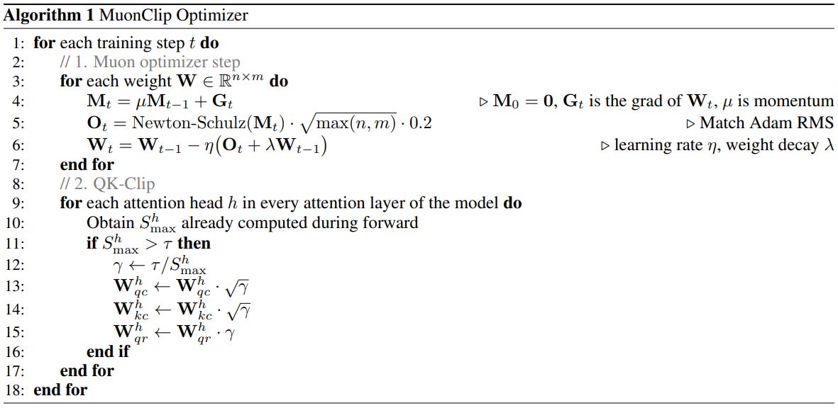
As we saw in the MLA section, we apply the decoupled RoPE strategy to Q and K by splitting Q and K both into two equal halves, C (compressed using Latent representation) and R (uncompressed, and hence RoPE is applied).
Similar to that, we apply clipping only on unshared attention head components:
References: