From Vanilla Transformers to Modern LLMs: What Changed After the Original Transformer (Part 1)

Modern LLM Architecture (Part 1): From Vanilla Transformers to Stable Training

This post is Part 1 of a 3-part series on modern LLM architectures. Each part can be read independently.

Part 2 talks about efficient architecture-level Attention Optimizations

Part 3 talks about low-level hardware attention optimizations and MuonClip Optimizer

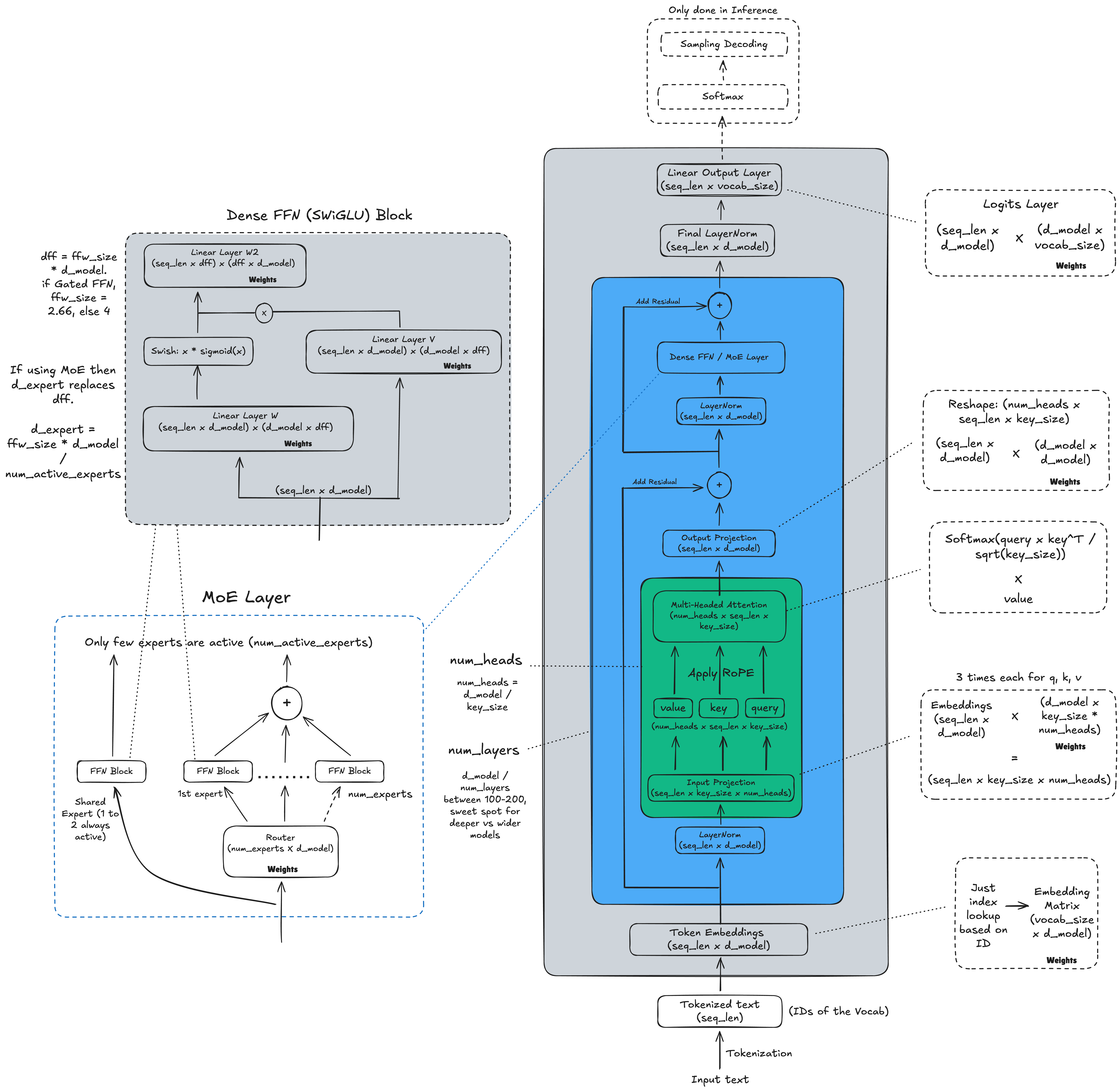
Let’s take a look at what modern LLM architectures actually look like today, and how they have diverged from the vanilla Transformer designs used just a few years ago.

Rather than a single radical redesign, progress has come from many small but compounding architectural improvements across normalization, attention, activations, memory efficiency, and optimization. Together, these changes enable today’s models to train more stably, scale further, and run far more efficiently.

1. Normalization Layer Placement: Post-Norm → Pre-Norm

Early Transformer models used post-normalization, where normalization was applied inside the residual stream and after the attention and FFN blocks.

Modern LLMs have almost universally moved to pre-normalization, where normalization is applied:

• Before the attention block

• Before the FFN block

• Outside the residual stream

This change has two major benefits:

1. Training stability
   Normalizing inputs before attention and FFN stabilizes activations and leads to smoother loss curves.

2. Improved gradient flow
   Keeping normalization outside the residual stream preserves the identity path, improving gradient propagation during backpropagation.

Better Validation Loss with Pre-Normalization as seen in the experiments from Xiong 2020

Fewer gradient spikes during training as per experiments from Salazar and Nguyen

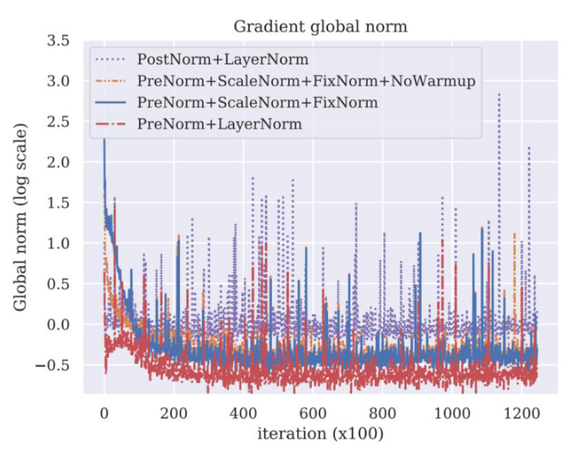
Today, virtually every LLM uses pre-normalization. Some architectures additionally apply a lightweight post-norm outside the residual stream for extra stability.

---

2. LayerNorm vs RMSNorm

LayerNorm learns two parameters per layer (scale and bias), while RMSNorm learns only one (scale).

Why RMSNorm won out:

• Fewer trainable parameters

• Less memory movement during inference

• Lower compute cost (no mean subtraction or bias addition)

\(\displaylines{ LayerNorm(x) = \gamma \odot \frac{x - \mu}{\sqrt{\sigma^2 + \epsilon}} + \beta \\ \\ RMSNorm(x) = \frac{x}{\sqrt{\frac{1}{n} \sum_{i=1}^{n} x_i^2 + \epsilon}} \odot \gamma }\)

As a result, most modern LLMs have adopted RMSNorm for both pre-norm and internal normalization (e.g., QK-Norm).

---

3. Activation Functions and the Rise of SwiGLU

Below is the graph of different activation functions mainly ReLU, GeLU, and Swish.

Early FFNs used ReLU, which suffered from dead neurons when activations went negative. This led to the adoption of GeLU and Swish, which preserve gradient flow.

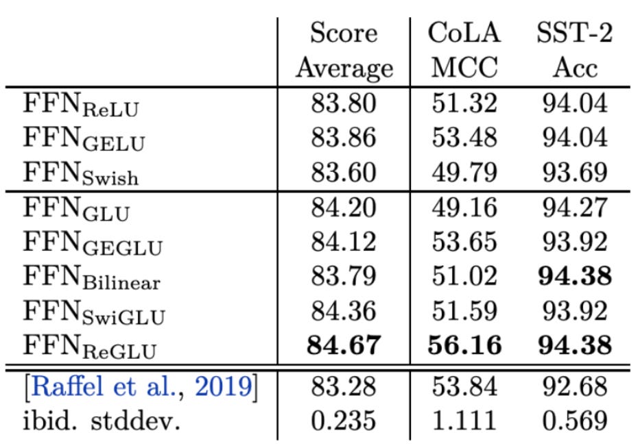
Modern LLMs go one step further with Gated FFNs, typically using SwiGLU, which consists of:

• Two up-projection matrices

• Element-wise gating

• One down-projection

To compensate for an extra up-projection compared to early FFNs, the intermediate dimension is reduced, keeping FLOPs roughly constant while improving expressiveness.

\(\displaylines{ FFN(x) = (\sigma(xW_{up}))W_{down} \\ GatedFFN(x) = (\sigma (xW_{gate}) \odot (xW_{up})) W_{down} \\ \\ Where, \\ \text{$\sigma$ is an activation function and $\odot$ is element-wise multiplication.} }\)

Empirical evidence (Shazeer et al., 2020) shows that Gated Linear Units consistently outperform standard FFNs, and they are now the default in most state-of-the-art models.

Shazeer 2020

---

4. Rotary Positional Embeddings (RoPE)

Earlier models used absolute positional embeddings (e.g., sinusoidal), where a vector e is assigned to each position of the input. It is added to the token embedding before the first attention layer:

\(h_{0}^{i} = W_{token}^{i} + e_{pos}^{i}\)

Problems with Absolute Positional Embeddings:

1. Fixed context length
   Positions beyond training length cannot be represented naturally.

2. No relative distance awareness
   The model treats position differences uniformly, regardless of actual distance.

Why RoPE Works Better:

RoPE applies position-dependent rotations directly to query and key vectors inside each attention head, rather than modifying token embeddings upfront.

Key advantages:

• Encodes relative position information naturally

• Enables length extrapolation

• Integrates cleanly into attention computation

In practice:

• Q and K vectors are split into 2-D pairs

• Each pair is rotated using position-dependent rotation matrices

• This is implemented efficiently without explicitly forming full matrices

Su et al 2021

\(\displaylines{ \text{Rotation Matrix } R(\theta) = \begin{bmatrix} \cos m\theta_{i} & -\sin m\theta_{i} \\ \sin m\theta_{i} & \cos m\theta_{i} \end{bmatrix} \\ \\ \text{Where,} \\ \theta_{i} = \frac{1}{w^{2(i-1) / d}} \\ \text{m = position of the token in the embedding vector} \\ \text{w = frequency (10,000 for example)} \\ \text{i = pair number (total d/2 pairs) [1, 2, . . ., d/2]} \\ \text{d = key_size (64 for example)} }\)

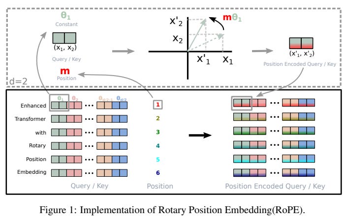
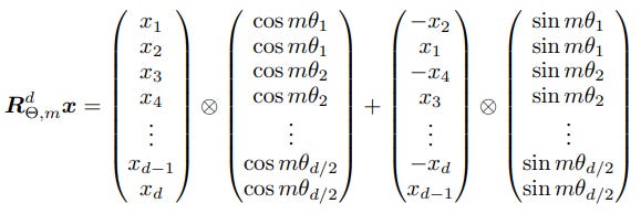
Query and Key matrix has the shape of (seq_len x key_size) as shown in the architecture figure at the start. Let’s say our “seq_len” = 5 (“Please check out this blog”). For the word “Please”, m = 1, d = 64. We divide the total “key_size” dimension into pairs of 2. Hence, for the indices 0 and 1 of the key_size dimension, we have the pair index i = 0, and so on.

The final computationally efficient realization of rotary matrix multiplication with query/key vector for the Mth position looks like this:

Su et al 2021

---

5. QK Norm

QK-Norm is a stability technique that normalizes query and key vectors inside each attention head before applying RoPE.

Why it matters:

• Prevents exploding dot-products in attention

• Enables higher learning rates

• Produces smoother training and validation loss curves

Among normalization choices (LayerNorm, RMSNorm, L2), RMSNorm again performs best in terms of efficiency and stability.

There are different variants regarding Normalization to improve the stability during pre-training and also reduce the perplexity, but QK_Norm performs the best of all, as shown in the research by Rybakov et al., 2024

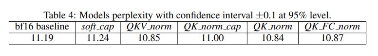
Recent work (Rybakov et al., 2024) shows that QK-Norm consistently reduces perplexity and improves convergence across language, vision, and translation tasks.

---

6. Per-Layer QK Norm

QK Norm is a stability technique that helps stabilize the training process as discussed in the earlier sections. This should not be confused with Pre-Normalization, which we do before passing the embedding to the transformer layers and projecting it into Q, K and V matrices.

In a standard setting of QK Norm technique, it is defined in each transformer block (or layer) and it is shared among the attention heads of that same layer. Just as Pre-Normalization, here also we can either use LayerNorm or RMSNorm. However, RMSNorm is preferred because of the reasons that we discussed earlier.

In Per-Layer QK Norm, the Normalization is defined in each transformer block(or layer) but it is not shared among attention heads. So it is different for each attention head.

---

References:

1. Rybakov et al 2024

2. Su et al 2021

3. Shazeer et al 2020

4. Xiong et al 2020

5. Salazar and Nguyen et al 2019

---

That was it for this Part. Next Part-2 will drop this weekend, so stay tuned!!

Quick Part-2 Teaser: Efficient Attention and Long Context

Content:

• MHA → MQA → GQA

• MLA (DeepSeek)

• Sliding Window Attention

• DeepSeek Sparse Attention

• Gated DeltaNet

• Gated SDPA

What are your thoughts about those changes compared to the vanilla transformer? Let me know in the comments!